5.1 Introduction
In chapter previous the structure of the model for the management of the supplyes has been studied under an unexpected increase
of 20% of the question that then remains constant.
The reaction of the system to this unexpected event is expressed in a sure delay of the answer of the variable ones in order to bring back
the same system to the equilibrium.
The scope of this chapter is that one to study the model, and therefore the answer of the variable ones that characterizes it,
under various conditions of variation of the question.
5.2 Chance variation of the question
In the real world, sure, the supply chains they are not hit only once but continuously they are disturbed from variations
of the orders of the customers.
These unexpected variations disturb the system carrying it outside from the equilibrium, provoking a characteristic answer
that constantly it depends on the structure of own feedback of the system.
A flow of chance variations in the question can be thought like a continuous succession of small pulsations
in the question, ognuna with one accidental largeness.
A time of simulation of a year is considered and that the several question accidentally in a range comprised between 10 and
12 widgets/week like brought back in the following diagram:
Figure 5.1- Chance variation of the question.
The diagrams of figure 5.2 show the answer of the system to one chance variation in the orders of the customer.
As one expects to us, the supply chain it is behaved playing like a door-bell.
Variable shipment the installments and desired shipment installments show this type of answer well.
In the first months of simulation desired shipment it oscillates above shipment because of forehead to a chance variation
of the question the company is found spiazzata initially and the warehouse comes down to of under of the wished level.
After approximately six months of simulation shipment and desired shipment they catch up the same level and delivery delay it returns to its
value begins them (2 weeks).
Beginning from this period until the end of the simulation shipment and desired shipment has the same course,
because the warehouse has caught up the wished level, and oscillates to the same way in a narrow range around
to the value of 11 widgets/week that it is the medium value between 10 and 12 widgets/week.
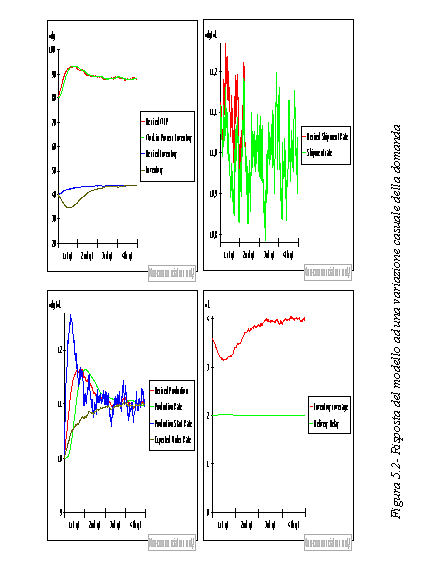
The difference between the warehouse puts into effect them and that one wished, caused from the accidental variation of the question forces production
start installments to increase with an amplification of approximately 40% regarding the value begins them (10 wdg/wk).
This increase has had to the fact that of forehead to a chance variation of the orders the company is not endured in degree
to plan one correct forecast of the orders of the customers.
In fact famous that after approximately six months the paramentri of the system only oscillates in a more and more narrow range
(around to the 11 widgets/week).
This evidences that the scope of the warehouse and the backlogs in a supply chain is that one
tamponare the system against unexpected fluctuations of the question, naturally with delays that depend on
the characteristics of the same system.
Of continuation the tables with the values assumed from the parameters of the system in the course of the simulation are brought back:
Figure 5.3- Table that filler the WIP, values inventory, desired inventory and desired WIP assumed during the simulation
Figure 5.4- Table that filler the values of production installments, customer order installments, expected order installments, desired production, production start installments, desired shipment installments, shipment installments assumed during the simulation